The Anatomy of MS Excel Spreadsheet
Excel Tutorial: BE02
The anatomy of MS Excel spreadsheet means the basic structure of Excel, what are its main components and where are their locations.
However, before we dig into the structure, let’s first understand the difference between an Excel sheet and an Excel workbook.
Excel sheet is a SINGLE page grid-like structure organized into rows and columns used for performing tasks, it is also known as an Excel spreadsheet.
Whereas an Excel workbook is a collection of multiple Excel spreadsheets. When you open Excel on your computer, you open an Excel workbook and within the workbook, you will have one or multiple Excel sheets.
Excel is one of the applications of Microsoft Office bundle, which is loaded to your computer. Here we will learn about the main parts of MS excel.
The Anatomy of Excel Spreadsheet
There are various components which are there in Excel, you will notice certain icons, text, and tabs on the face of the Excel sheet. What are all these icons for? Let’s understand them all one by one.
Once you open Excel by following any method as mentioned in Course Module BE01 in your system, you will notice three prominent areas in Excel.
- Areas with icons and buttons at the top
- Grid-likestructure having rectangular boxes in between.
- Plain bar-like structure at the bottom.
In this Module, we will make you conversant with every part of Excel.
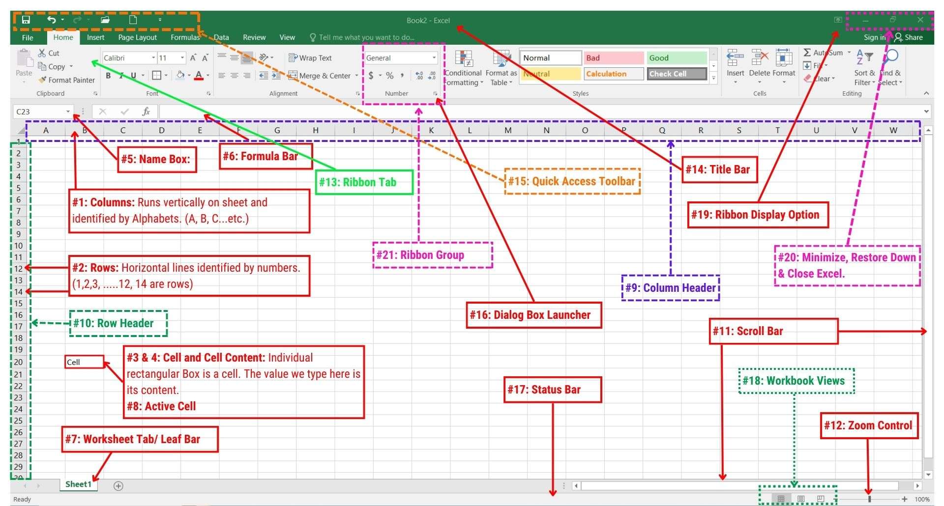
The structural parts of the Excel are explained below:
1. Columns: Columns run vertically on the sheet and are identified by alphabets or you can also say English letters such as A, B, C, etc., at the top of the sheet. Each column represents a unique vertical data set.
2. Rows: Rows are horizontal lines or we can say row of boxes that runs horizontally on the Excel sheet are called rows. These rows are represented by Numerical values such as 1, 2,3, etc.
These numbers are present at the extreme left of the Middle part of the Excel sheet. Each row represents a unique horizontal data set.
3. Cells: Cells are individual rectangular boxes formed by the intersection of rows and columns. Each cell has its unique address which is Column Alphabet and Row Number.
This unique cell address of the active cell you can see in the Name Box. It will have a column letter first followed by a row number.
Example: If you have selected a cell in Column B and Row number 5 then the Unique Address of your selected cell is B5.
4. Cell Content: The values you supply to the cell are called cell content. The content of a cell can be of various types of data, it could be numbers, text, dates, formulas, or functions. You can enter, edit, or delete cell content.
5. Name Box:The name box represents the location of the active cell, which means
- It will show you the location address of the cell where you have placed your cursor or the selected cell.
- It also represents the address of the cell where values are present.
6. Formula Bar: The formula bar, located just below the toolbar, displays the contents of the active cell. It will display the contents or values of the selected cell. In case formulas are applied to any cell and when you place the cursor over it, means when you select it, it will give the entire formula in the formula bar.
7. Worksheet Tabs: At the left bottom of the Excel window, you will find worksheet tabs. This tab shows the names of sheets present in the Excel workbook.
You can create multiple sheets in a single workbook. The sheet that you are working on (active sheet) will become transparent white while other sheets will become grey by default (although you can change the color of the sheets, rename, move, and delete them though).
8. Active Cell: The active cell is the cell you are working on or you have placed your cursor on. Wherever you type your content will become the active cell.
9. Column Header: The top column of the sheet containing all the column names that as A, B, C… etc., is called as column header. It helps in identifying the location of the data in the sheet.
10. Row Header: The left-most vertically arranged row numbers 1, 2, 3, etc., serve as row headers in the Excel spreadsheet. They help in identifying the location of specific data in the sheet.
11. Scroll Bars: Since there are lot many rows and columns that display on the computer screen, or we can not fit all the rows and columns of the Excel sheet on our computer screen, we have scroll bars present at the right-most side of Excel and at the bottom of the excel.
These scroll bars are there to scroll the rows and columns to see the data values displayed in the window.
These vertical and horizontal scroll bar is to navigate the Excel sheet and nothing more.
12. Zoom Control: At the bottom right of the Excel sheet we have the Zoom control function. This is used to increase (Zoom in) the size of the grid boxes and to decrease the (Zoom out) size of the grid boxes.
The zoom-in and zoom-out work as a lens; it increases the view not the actual size of the data present in the sheet.
This means if you have entered Value “Apple” in a font size of 12, at a zoom-in percent of 100%, and then if you increase the zoom-in percentage to 120%. The Value “Apple” will appear large, however, its actual size remains font size 12 only.
Zoom in and Zoom out does not make any difference when you print the document. The size remains the same it (zoom in) only makes things look closer and nothing else.
13. Excel Ribbon: Excel has a ribbon at the top of the window, which contains various tabs with commands for formatting, data manipulation, and other functionalities.
By default, in Excel, you will normally have a Home Ribbon tab, an Insert Ribbon tab, a Formula tab, a Data tab, a Review tab, and a View tab.
You can always customize and create custom Excel ribbon as per your requirements.
14. Title Bar: At the top of the Excel you will see the name of the workbook followed by Excel. This top bar is called the title bar in Excel.
The title bar contains the saved file name of an Excel workbook.
For example, if you create a new workbook and save it with the name “Learning Excel Formula” then this name will appear in the title bar whenever you open this (Learning Excel Formula) file.
15. Quick Access Toolbar: At the extreme top left you will a toolbar, called as Quick Access Tool Bar. In this toolbar, we have can commands that are most frequently used while working with the Excel sheet. We can customize the quick-access toolbar as per our requirements.
The most common commands present in Excel 2016 are New, Open, save, email, quick print, print, preview, and print, Spelling, undo, redo, sort ascending, sort descending, touch/mouse mode, and save below ribbon.
16. Dialog box Launcher: In the Excel ribbon tab we have multiple command groups containing similar types of functions and if there are more functions within that command group then those are not directly visible to the users.
To view those hidden extra options, we need to click a small icon present at the bottom right of the command group. This small icon is called a dialog launcher, as it launches other related options associated with that command group.
17. Status Bar: The status bar is present at the bottom of the Excel window which displays important information related to the working status of Excel. The status bar has multiple options to be displayed on this bar which can be viewed by right clicking the mouse on the status bar.
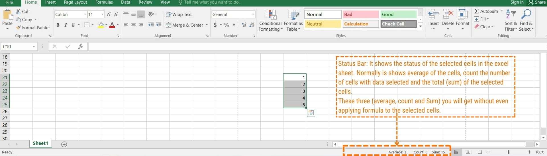
Example: If we select five cells with values ranging from 1 to 5 then we can see the average, count, and sum of these digits (selected cells) in the status bar even without performing any calculation in the Excel.
18. Workbook Views: Workbook views are a group of three small buttons present at the right bottom of the Excel windows between the status bar and zoom control. The main function of the workbook views buttons is to display the workbook in three different forms.
The three different forms of display are:
- Normal View: This is the first button of the workbook view buttons; this displays the workbook in the normal view.
- Page Layout View: The middle button of the workbook view is the page layout view which has the option to arrange the Excel in a way you would do with a Word document file. This means you can apply section breaks, indentation, and page number, and add header footer and orientation before applying the final printing to the document.
- Page break Preview: The last button of the workbook view is of page break preview. It has the functionality to insert, move, and remove page breaks from the documents. This helps in preparing the document before giving the final print to the document thus preventing the wastage of papers.
19. Ribbon Display Option: At the top right of the Excel window you will see the arrow icon within a box. This button has three options related to Excel Ribbon:
- Auto Hide Ribbon: This option will hide the Excel Ribbon completely from your screen.
- Show Tabs: This option will show only the name of the ribbon tabs without the ribbon commands.
- Show Tabs and Commands: This option will display ribbon tabs along with the commands all the time on the Excel header.
20. Minimize, Restore Down, Close: At the top right of the Excel group three buttons are available, these are the most common buttons present in most of the internet applications.
Minimize: This will minimize the window and just display the icon in the taskbar. This means your application is open, whoever, it has been minimized in its view.
Restore Down: The restore down button is used to reduce the window size from its maximum size. This helps in moving and arranging the window anywhere on the screen.
Close: This is cross-size symbol present at the extreme top right of the window, and it is used to close the application. If the task on the active sheet is saved the application will close without any notice else it will ask to save the changes made to the workbook.
12. Ribbon Group: Ribbon group consists of a set of closely related commands in Excel ribbon which are used to perform a task of a broader category.
This module helps learners to become conversant with the anatomy of MS Excel Spreadsheet. Familiarity with the Excel Graphical User Interface (GUI) is essential to the progress journey of Excel proficiency.
Thanks for reading!
Happy Learning,
Team Excel Hippo.
About the Author: Excel Hippo