Excel Tutorial: Insert Ribbon Tab
Tutorial Code: BE07
Introduction:
The “Insert” ribbon tab in Microsoft Excel, by default is located at the 3rd position in the top header of the Excel window. The “Insert” tab provides various options for adding different elements to your Excel workbook, inserting pivot tables, various types of charts, tables, pictures, shapes, and many more.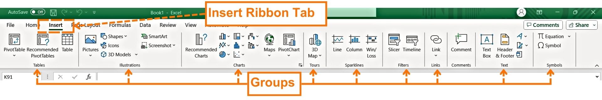
This course module will make the candidate well aware of the structure and features present in the Insert Ribbon Tab. In this module, we have explained all the groups, their features, and all the command buttons available on the face of the Excel Workbook.
Here is the list of all the groups present in the Insert Ribbon Tab of Excel application of Microsoft 365:
- Tables
- Illustrations
- Charts
- Tours
- Sparklines
- Filters
- Links
- Comments
- Text
- Symbols
1. Tables
Tables: This group allows you to insert tables into the worksheet. Tables provide a structured way to organize and manage data, and they come with additional features like filtering and sorting.
The main buttons available in the Table group are:
- Pivot Tables
- Recommended Pivot Tables
- Tables
To locate the “Tables” group in MS Excel, follow this path:
Insert > Tables.
Keyboard Shortcut Key for tables: Alt + N
Below is the details of each command button of the Tables group:
A. Pivot Tables:
This option allows users to create a Pivot Table based on the data present in the Excel sheet. It makes it easier to analyze and summarize the data from the larger data sets.
The pivot table command provides flexibility to the users to create another table based on the existing tables or data sets so that users can arrange the fields according to their choice without changing the structure of the original tables.
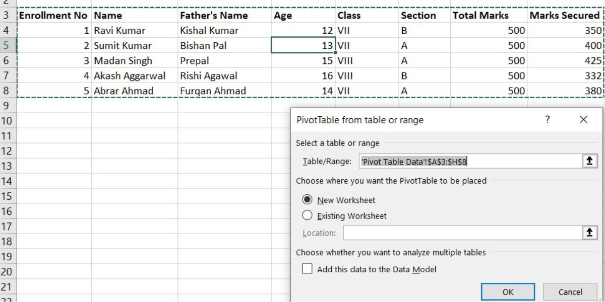
Select the range or table within your data, then click the “PivotTable” button, Choose where you want the PivotTable to be placed, and define its structure in the PivotTable Field List.
We are covering here only one example to explain how to apply or create a pivot table from the data set/Table present in the Excel sheet, it will take an entire module to explain all the functions associated with it.
In the below example, we have explained how to create a pivot and its design from the simple data table.
How to apply the Pivot Table command?
Here is a simple example of applying the pivot table command.
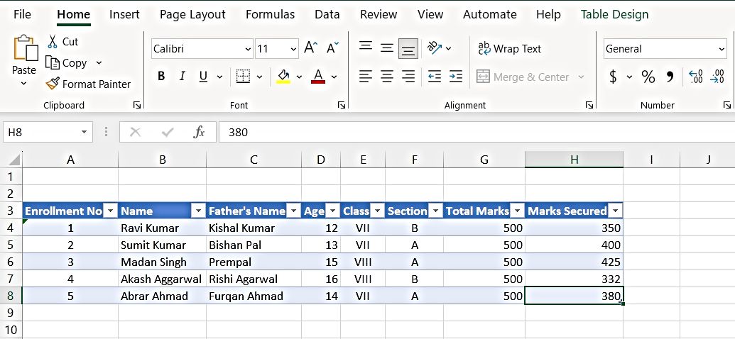
- Let’s take the data present in the table shown in Table #1.
Insert Image of data table present in the “Modules and web codes” workbook in pivot data table sheet.
Image: Table #1
| Enrollment No | Name | Father’s Name | Age | Class | Section | Total Marks | Marks Secured |
| 1 | Ravi Kumar | Kishal Kumar | 12 | VII | B | 500 | 350 |
| 2 | Sumit Kumar | Bishan Pal | 13 | VII | A | 500 | 400 |
| 3 | Madan Singh | Prempal | 15 | VIII | A | 500 | 425 |
| 4 | Akash Aggarwal | Rishi Agarwal | 16 | VIII | B | 500 | 332 |
| 5 | Abrar Ahmad | Furqan Ahmad | 14 | VII | A | 500 | 380 |
Tables: This group allows you to insert tables into the worksheet. Tables provide a structured way to organize and manage data, and they come with additional features like filtering and sorting.
The main buttons available in the Table group are:
- Pivot Tables
- Recommended Pivot Tables
- Tables
To locate the “Tables” group in MS Excel, follow this path:
Insert > Tables.
Keyboard Shortcut Key for tables: Alt + N
Below is the details of each command button of the Tables group:
A. Pivot Tables:
This option allows users to create a Pivot Table based on the data present in the Excel sheet. It makes it easier to analyze and summarize the data from the larger data sets.
The pivot table command provides flexibility to the users to create another table based on the existing tables or data sets so that users can arrange the fields according to their choice without changing the structure of the original tables.
Select the range or table within your data, then click the “PivotTable” button, Choose where you want the PivotTable to be placed, and define its structure in the PivotTable Field List.
We are covering here only one example to explain how to apply or create a pivot table from the data set/Table present in the Excel sheet, it will take an entire module to explain all the functions associated with it.
In the below example, we have explained how to create a pivot and its design from the simple data table.
How to apply the Pivot Table command?
Here is a simple example of applying the pivot table command.
- Let’s take the data present in the table shown in Table #1.
Insert Image of data table present in the “Modules and web codes” workbook in pivot data table sheet.
Image: Table #1
Click on the “Pivot Table” dropdown button and select “from Table/Range” from the dropdown options.
- A new dialog box will open, asking to select the table range. Select the entire table as shown in the Image: Table #1, and then select one of the options “Choose where you want the pivot table to be placed”. Better to select the new sheet. Click OK.
- It will create a new sheet along with the Pivot field options on the right-hand side of the sheet.
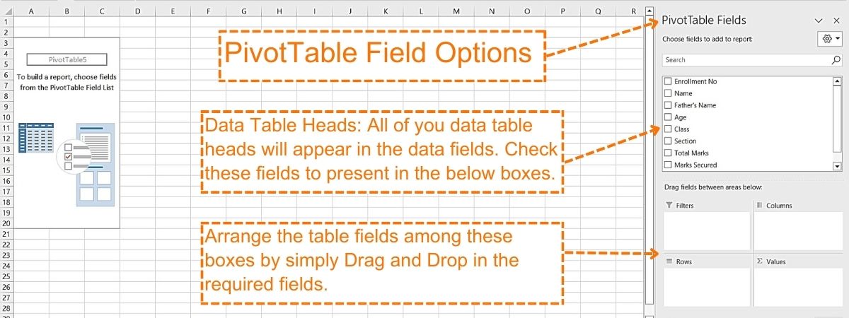 Image: Pivot Field Options
- Select the fields of your choice from the “Pivot Table Fields” and then arrange them in required cells “rectangular sections” represented as Filter, Columns, Rows, and Values. Your data won’t fall automatically in these cells, you must drag and drop in these square boxes. Arrange it as shown in the image below.
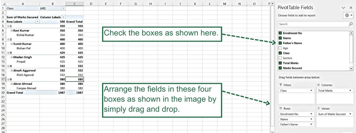 Image: Field selections
- Now the last part is designing the report.
- Once your pivot table is created, automatically extra tabs are created on the top Excel header to add additional functionality to pivot tables. These tabs are:
- PivotTable Analyze
- Design
Now let’s discuss the design part of Pivot Tables:
To design a report something to look like the image below:
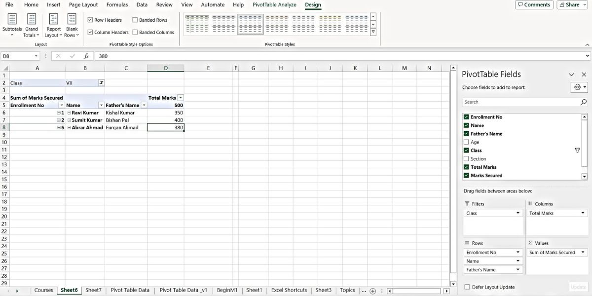 Image of the Report design
Step 1: Click on the “Design” tab created at the header once you create a Pivot table. And Go to the “Layout” Group of the design tab.
Step 2: Click on the dropdown button present in the “Grand Total” button and select “Off for
Rows and Columns.”
Step 3: Click on the dropdown of the “Report Layout” button and select the “show in tabular form” option.
Step 4: and finally, Click on the dropdown of the “Subtotal” button and select the “Do Not Subtotal”
Step 5: Your report is ready.
To locate the “Pivot Tables” group in MS Excel, follow this path:
Insert > Tables.> Pivot Tables
Keyboard Shortcut Key for Pivot Tables: Alt + N + V
B. Recommended PivotTables:
This function helps users to use the already built Pivots that Excel feels are best for your data set. Once you select this button a new dialog box opens with a customized set of PivotTables to arrange your data.
To locate the “Recommended PivotTables” group in MS Excel, follow this path:
Insert > Tables.> Recommended PivotTables
Keyboard Shortcut Key for Recommended PivotTables: Alt + N + SP
C. Tables:
This option helps users create a table in a customized template to organize and analyze table data in a better way. This customized table helps users to easily sort and filter data.
Sample table prepared by using the “table” option.
To prepare formatted table data as shown in the above image follow these steps:
Step 1: Select the entire data/Table preset in the Excel sheet.
Step 2: Click the “Table” command button/Icon. A small dialog box will open, check the “My table has headers” box and click OK.
Step 3: Automatically it will create a table with a header. It’s so simple.
Step 4: A new table with a header is created. It’s so simple.
Note: Once you create a table using the “Table” button, you will notice a new tab “Table Design” is created at the top header of the Excel. This is used to apply styles to your newly created table.
To locate the “Table” button in MS Excel, follow this path:
Insert > Tables.> Table
Keyboard Shortcut Key: Ctrl + T
2. Illustrations
Illustrations: The “Illustrations” group of the “insert ribbon tab” offers options to insert various graphical elements, such as pictures, online images, shapes, smart art, and icons in the Excel workbook.
- Pictures: Insert pictures from your desktop and other online resources.
Keyboard Shortcut Key to insert Pictures: Alt, N, P
- Shapes: Insert various types of readymade shapes present in MS Excel, such as circles, triangles, squares, etc.
Keyboard Shortcut Key to insert shapes: Alt, N, SH
- Icons: Insert various types of icons from the vast array of subjects, such as toys, animals, emojis, etc.
Keyboard Shortcut Key to insert icons: Alt, N, NS
- 3D Models: Insert various types of animated 3D models, such as toys, animals, etc. which can be rotated so that users can see those from all angles.
Keyboard Shortcut Key to use 3D models: Alt, N, S3
- Smart Art: Insert the SmartArt graphic into the spreadsheet to add a visual effect to the communications.
Keyboard Shortcut Key to use smart arts: Alt, N, M1
- Screenshot: This command helps users insert the screenshot of the window that is open on the desktop to the spreadsheet.
Keyboard Shortcut Key to insert screenshots: Alt, N, SC
3. Charts
Charts: This group allows users to represent data in a graphical format. It creates different types of charts based on the data present in the Excel workbook. Different types of charts can be created in Excel, such as column charts, pie charts, line charts, bar charts, and more. Charts are powerful tools for visualizing and analyzing data trends.
When you select the data and click on the dropdown arrow of the “Chart” group of the Insert Ribbon tab, a new window will open with two tabs, A) Recommended Charts and B) All Charts.
A) Recommended Charts: This feature helps in recommending the best chart for the data present in Excel.
Example 1: Let’s consider data from Table No. 1 to apply the “Recommended Charts” function for creating a chart.
Table No 1
Once we select the data and press the “recommended chart” option, a window will open with the chart recommendations.
Keyboard Shortcut for Recommended Charts: Alt, N, R
Excel has recommended four chart types for this data, see the image below, The Excel recommended chart types are clustered column, Pie chart, Clustered bar, and Funnel chart type.
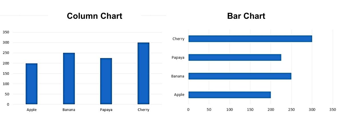
B. All chart Types: There are 8 different icons representing all the chart types present in MS Excel (Microsoft 365). We are creating each type of chart using data from table No.1 (above)
1.Column or Bar Chart
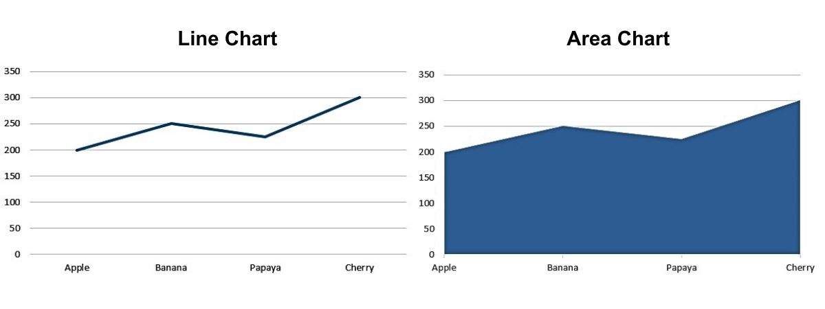
2. Line or Area Chart
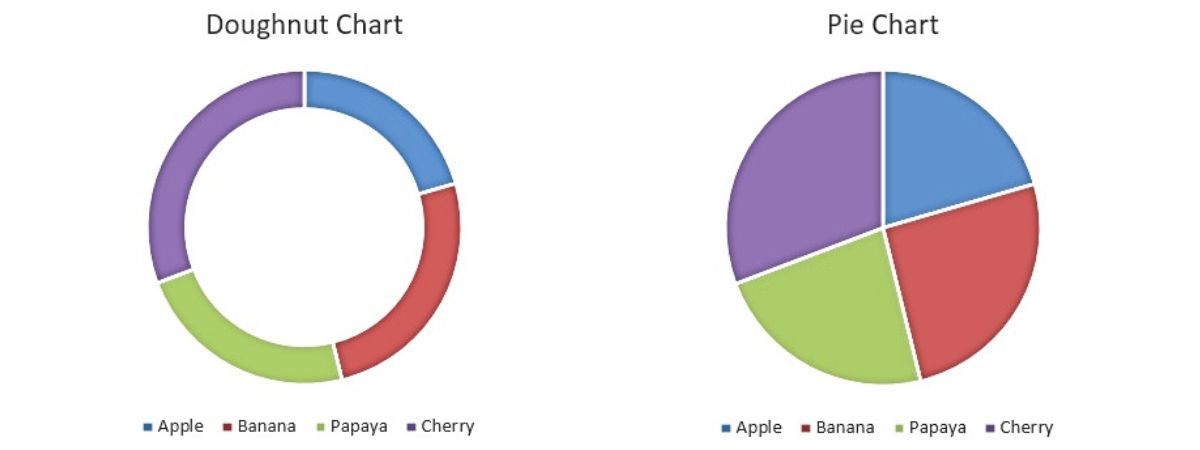
3.Pie or Doughnut Chart
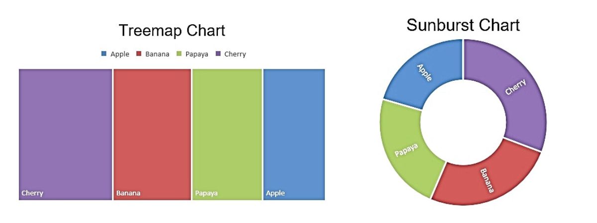
4.Hierarchy Charts:
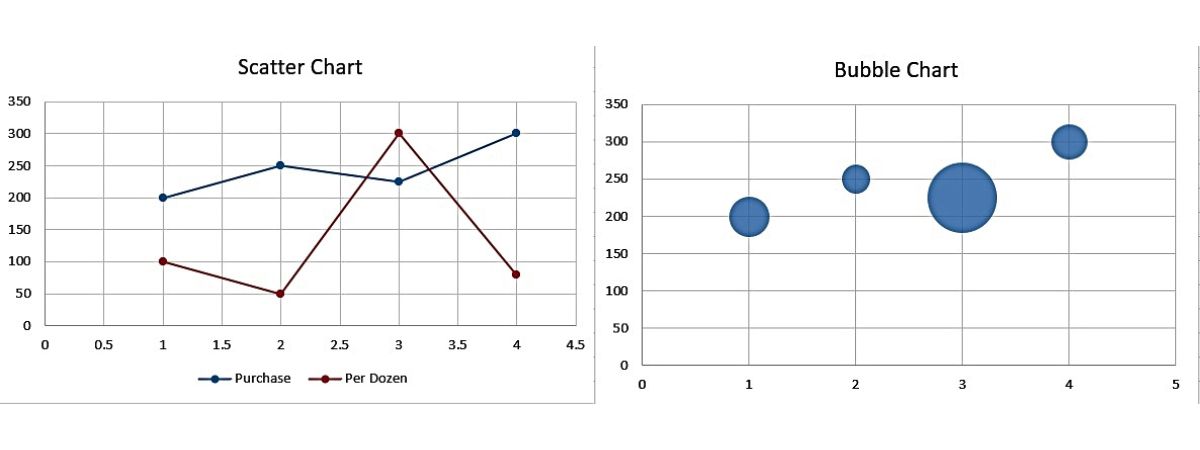
5.Scatter or Bubble Chart: These types of charts are used to show the relationship between different sets of values. In scatter chart is prepared when the data represents the separate measurements. Whereas a bubble chart is prepared to compare at least three sets of data values and a third is normally used to determine the relative of the bubble.
6. Waterfall, Funnel, Stock, Surface, and Radar
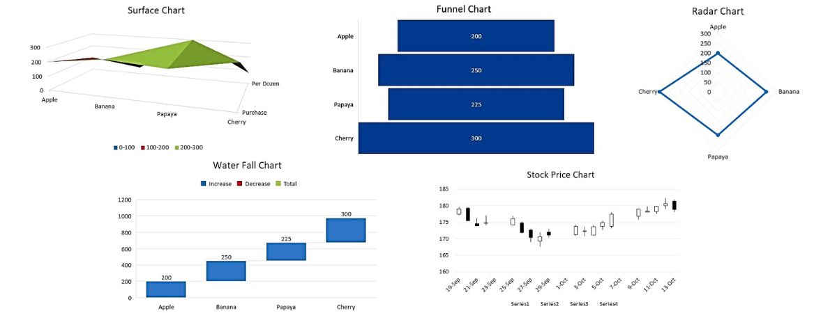
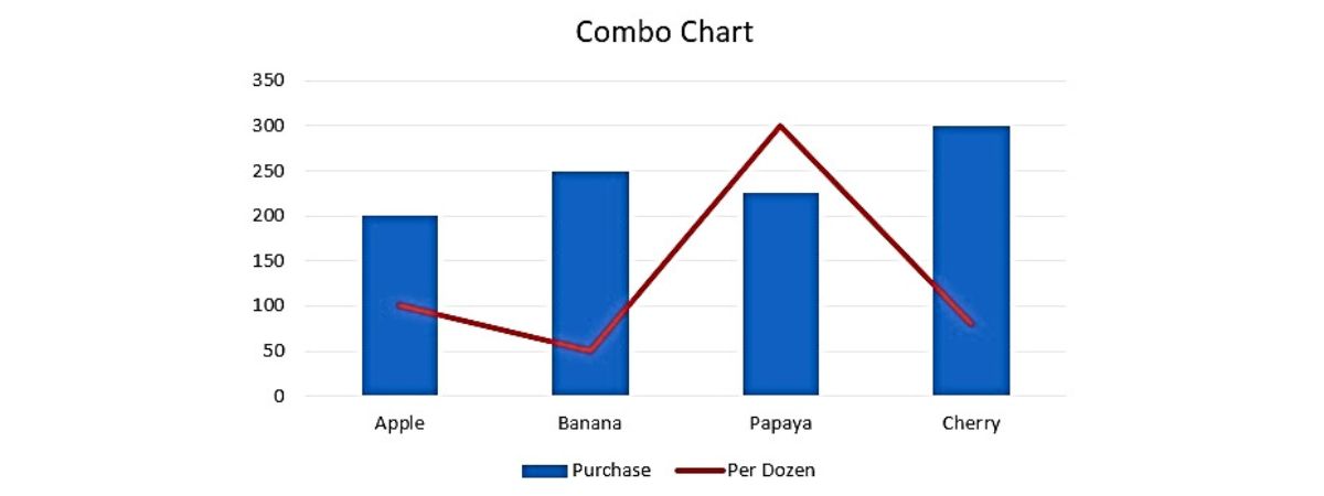
7. Combo
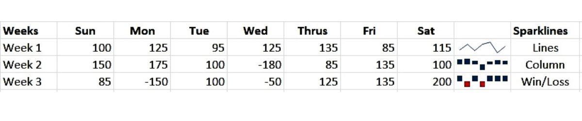
4. Sparklines
Sparklines are small, simple charts that fit within a single cell, and they are used to show trends or patterns present in the selected data set. This group provides options for inserting sparklines in the cells of the spreadsheet.
There are 3 types of sparklines present in the MS Excel of Microsoft 365.
- Line
- Column
- Win/Loss
Here is the image depicting all three types of sparklines:
To draw sparklines, click on the button of your choice to select the sparkline, it will ask for two options:
- Choose the data that you want to create sparklines for: Select the range of cells for input data.
- Choose where you want the sparklines to be placed: Select the location where sparklines are to be displayed/created.
To locate the “Line” type of Sparkline in MS Excel, follow this path:
Home > Sparklines> Line
Keyboard Shortcut Key for Line Type Sparkline: Alt, N, SL
To locate the “Column” type Sparkline in MS Excel, follow this path:
Home > Sparklines> Column
Keyboard Shortcut Key for Column type Sparkline: Alt, N, SO
To locate the “Win/Loss” type Sparkline in MS Excel, follow this path:
Home > Sparklines> Win/Loss
Keyboard Shortcut Key for “Win/Loss” type Sparkline: Alt, N, SW
5. Filters
Filters: This group contains commands for visually filtering data in tables. You can create filter criteria to display only specific data that meets certain conditions.
- Slicer: It is used to filter the data visually in a quicker and easier form. It helps in filtering data from Tables, Pivot Tables, and Pivot Charts. In simple words, the slicer creates small window boxes of filters to make it easier for the user to analyze and interpret data.
For instance, if you wish to apply a slicer to the pivot table, just click on the pivot table and click on the “slicer” button/Icon. A new window will open containing all the headers of the data set/Table on which you would like to create a filter, or you can say how many slicers you would like to create.
Once you check ticks on the boxes in the “insert slicer” window, you will notice an individual slicer is created for each selected table head.
To locate the “Slicer” command in MS Excel, follow this path:
Home > Filters> Slicer
Keyboard Shortcut Key for Slicer: Alt, N, SF
- Timeline: This command is used to filter the data with dates in an interactive mode. It makes it easier and faster to filter out time/Period data from Pivot Tables, Pivot Charts, and cube functions.
To locate the “Timeline” command in MS Excel, follow this path:
Home > Filters> Timeline
Keyboard Shortcut Key for Timeline: Alt, N, ST
6. Links
Links: The “Links” group allows you to insert hyperlinks to other files, web pages, or specific locations within the workbook.
- Hyperlink: Hyperlink is used to create a link in the workbook for quick access to the files in a folder, any sheet within the same workbook, webpages, and email addresses.
Here are the simple steps to insert hyperlinks:
- Select the content on which hyperlinks need to be inserted.
- Click on the “Link” icon and select the “Insert Link” command.
- A new window will open with options to link to:
- Existing file
- Place in this document
- Create a new Document.
- Email – Address
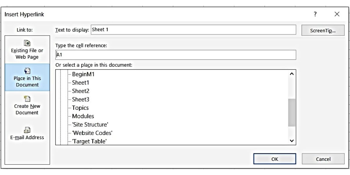
- Select the option, let you select “Place in this document” Then you will see all the sheets of your workbook in the window, and select the sheet that you want to link with the text.
- Click OK. You will notice that the cell/Content with hyperlink turns blue. Which means Hyperlink is added to your cell/content.
To locate the “Hyperlink” command in MS Excel, follow this path:
Home > Insert> Links>link>Insert Link
Keyboard Shortcut Key for Hyperlink: Alt, N, I2, I
7. Comments
Comments: This group contains only a single command button, and it is used to add comments or Notes to the selected cell.
To locate the “Comments” command in MS Excel, follow this path:
Home > Insert> Comments
Keyboard Shortcut Key for Comments: Alt, N, C2
9. Text
Text: The text group of “Insert Ribbon Tab” helps users to insert a text box, header & footer, WordArt, and object such as a PDF file, or Word document in the Excel spreadsheet.
A. Text Box: This is used to add a text box to include text within your worksheet.
To locate the “Text Box” command in MS Excel, follow this path:
Home > Insert> Text>Text Box
Keyboard Shortcut Key for Text Box: Alt, N, X
B. Header & Footer: This feature is used to insert the Header and Footer in the Excel spreadsheet, which customizes the Excel page for printing.
To locate the “Header & Footer” command in MS Excel, follow this path:
Home > Insert> Text> Header & Footer
Keyboard Shortcut Key for Header & Footer: Alt, N, H1
C. Insert WordArt: This command is used to insert WordArt in the document to give artistic flair to the spreadsheet.
To locate the “Insert WordArt” command in MS Excel, follow this path:
Home > Insert> Text> Insert WordArt
Keyboard Shortcut Key to insert word art: Alt, N, W
D. Add Signature Line: This feature provides users with the ability to add the signature line of an individual who must sign the document.
To locate the “Add Signature Line” command in MS Excel, follow this path:
Home > Insert> Text> Add Signature Line
Keyboard Shortcut Key: Alt, N, G
E. Object: This feature is used to insert some objects or files such as Word documents, other Excel workbooks, or PDF documents into the Excel workbook. This makes it easier for the users to keep all the embedded files in a single document.
Here are the steps to embed Word document [object] from your desktop into the Excel file:
Step 1: Go to the Insert tab and click on the “object” icon present in the “text” group. A new window will open that has two tabs,
a. Create New
b. Create from file.
Step 2: Click on the “Create from File” tab and browse you file already present in your system.
Step 3: Select the file and click the insert button. Check the button “Display as Icon” to display the file icon on your spreadsheet. Click OK.
Step 4: A small icon of Word doc will be displayed, if you click on this icon your embedded file will open.
To locate the “Object” command in MS Excel, follow this path:
Home > Insert> Text> Add Object
Keyboard Shortcut Key: Alt, N, J
10. Symbols
The Symbol group helps in inserting mathematical equations and special symbols in the spreadsheet.
This contains two command buttons:
A. Equation: This button helps users insert some of the most common mathematical equations in text format into the spreadsheet. These equations are an area of a circle, binomial theorem, expansions of a sum, Pythagoras theorem, etc.
To locate the “Equation” command in MS Excel, follow this path:
Home > Insert> Text> Equation
Keyboard Shortcut Key: Alt, N, E
B. Symbol: This button helps you to add some special symbols that are normally not present on the keyboards. This includes currency, micro sign, alpha, beta, gamma, etc.
These special symbols have their Unicode name and a character code.
Example: Symbol α (alpha) has Unicode name: Greek small letter alpha, character code as 03B1.
To locate “Symbol” command in MS Excel, follow this path:
Home > Insert> Text> Symbol
Keyboard Shortcut Key: Alt, N, U
About the Author: Excel Hippo