How To Wrap Text In Excel

Introduction:

This Excel Tutorial is intended to train Excel Beginners on how to wrap text in Excel, its application, and what possible issues arise with the warp text function.

Let’s proceed step by step starting with the meaning of the wrap text function.

Wrap text is a formatting option available in the Microsoft Excel application that allows the display of the contents of cells on multiple lines within a single cell without changing the column width. This functionality helps users to view all the information within a single cell and prevents the information from being overlooked.

Cell contents can take three formats in Excel these are Overflow, wrap text, and shrink to fit. The wrap text function automatically adjusts the row height to adjust the cell contents so that it can be read easily by the users.

Example 1: Here are the images showing the text within the Cell before and after the wrap text.

Image 1: Shows text before the application of wrap text functionality.

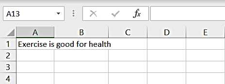
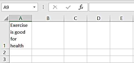
Image 2: Shows text before the application of wrap text functionality.

Wrap text is a command present in the Alignment Group of the Home Ribbon Tab of Excel Workbook.

Here are 5 ways to do the Wrap text in Excel Workbook:

1. Single Cell: Use the Format Cell option by right-clicking on the cell
2. Ribbon Option: Using the Command button option present in the Alignment Group
3. Alignment Dialog Launcher: Use the Alignment Group Dialog launcher to open the Format Cell Window
4. Line Break Option: Manually entering line break with the line
5. Keyboard Shortcut Option: Use of shortcut keys

Let us explain each of these options with the help of practical examples.

1. Single Cell:

This option is applied directly to the cell by right clicking the mouse button. Here are the simple steps to follow:

a. You can go to the cell where you’d like to do the text wrap. Let there be text in cell A1, as shown in the image below.

Select Cell A1

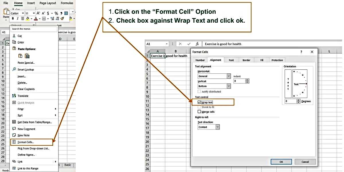
b. Right-click and select the “Format Cell” Option. See the left side of the image below. A ‘Format Cell’ window will open.

c. In the ‘Format Cell’ Window, check the box against the ‘wrap text’ option. See the right side of the image below.

2. Ribbon Option:

The Ribbon option for wrapping text in Excel is straightforward. Here are the simple steps to follow:

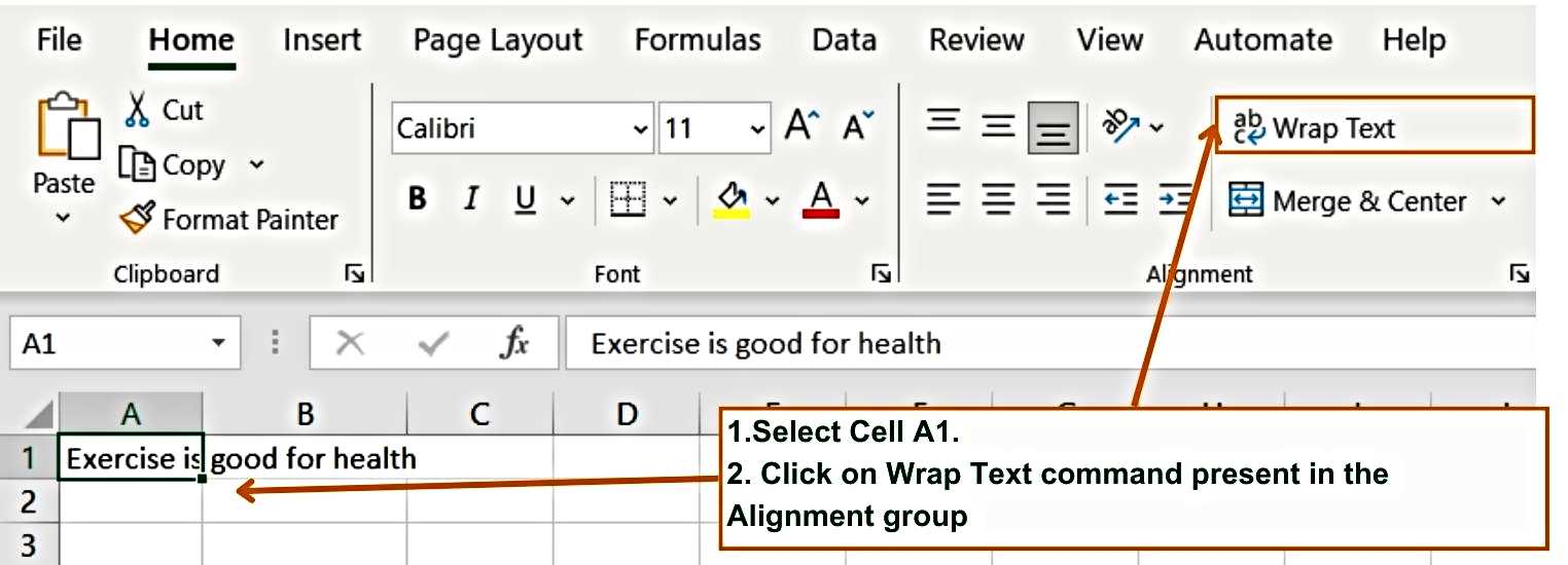
a. Select the required cell where wrapped text needs to be applied. Let us use the above example.

Select the Cell A1

b. Go to ‘Alignment Group’ and click on the ‘Wrap Text’ Command button. See the image below.

3. Alignment Dialog Launcher:

To wrap text using the alignment dialog launcher follow the steps given below:

Step 1: Go to Cell A1

Step 2: Click on the Alignment dialog launcher. See the image 7 below.

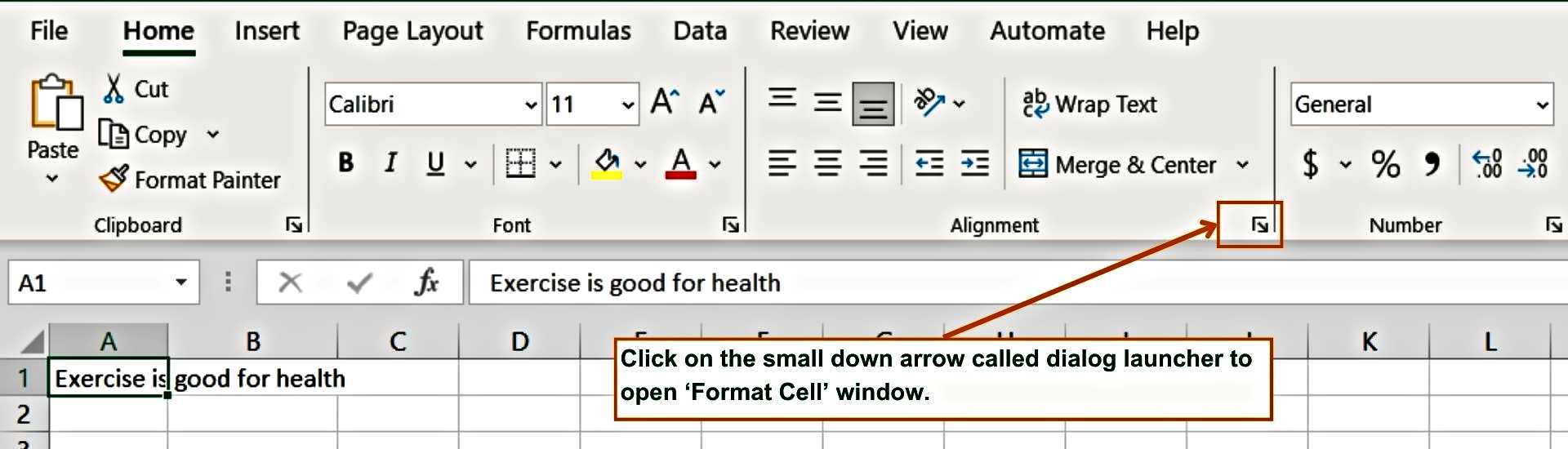
A new ‘Format Cell’ window will open.

Note: You can also open the ‘Format Cell’ windows by pressing CTRL + !

Step 3: In the Format Cell window, check the box against the ‘Wrap Text’ command. See the image below.

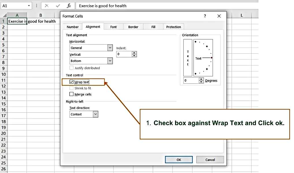
Step 4: Click OK

4. Line Break Option:

This is a manual feature to perform wrap text in Excel. It is done by inserting the line break with the contents of the cell.

Here are steps to manually perform wrap text using the line break option:

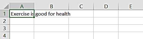
Example 2: Let us have a Text in Cell A1, ‘Exercise is good for health’ and We would like to apply a line break after ‘good’.

Step 1: Move your cursor to Cell A1.

Note: To enter the line break within the contents of the cell, first you need to place your mouse within the contents of the cell. This can be done by two methods:

a. Using the F2 Key on the keyboard.
b. By double-clicking the mouse (left double click) on the Cell.

Step 2: Press F2 OR double-click on Cell A1.

Step 3: Move the cursor after ‘good’ with the help of the arrow key. See image 9 below.

Step 4: Press ‘ALT + Enter’ (Together OR Keep Pressing the ALT Key and then press ENTER)

Step 5: Press Enter

5. Keyboard Shortcut Option:

You can use the wrap text feature using the keyboard keys, and there are shortcut keys for two methods mentioned above, one is for the Ribbon Option and the second is for the Single Cell option.

Wrap text keyboard shortcut keys for Ribbon Option:

Shortcut: ALT + H + W

Single Cell Option: To use the format cell option to wrap text in Excel you need to use a series of shortcut keys.

Step 1: Shortcut for format cell: CTRL + 1 (this will open Cell Format Windows)

Step 2: Go to Alignment and Press: ALT + W

It is super easy to use the wrap text feature in Excel, however, sometimes you may encounter issues and this feature may not work as desired.

There could be several reasons why the Wrap Text feature may not work, let’s explore some of the possible reasons here:

1. Width of the Column:

If the width of the column is more than the length of the text (Content), then the wrap text option seems like it is not working.

2. Fixed Height of Row:

If the height of the row is fixed to a level below the default level of Excel then the wrap text feature won’t work properly. Normally by default the height of the is 24 pixels OR 14.40 at Calibri font and font size of 11.

So, if you fix the row height at 15 or below, the wrap text won’t be displayed on the screen.

To avoid such issues, you must activate the “Autofit Row Height” feature. Follow the below path to activate the Autofit Row Height Feature.

Home > Cells > Formats > Autofit Row Height

11. Image: Shows the path to the “Autofit Row Height” feature

3. Two or more Cells are merged:

Another possible reason why the wrap text feature won’t work in Excel is if you have content in the merged cells.

Therefore, you must check if the cells are merged or not. If you find that content is present in the merged cells, then before applying the wrap text feature make sure you unmerged the cell first.

4. Horizontal Text Alignment is set to fill:

Let’s understand where we need to check whether Horizontal Text alignment is set to fill.

Step 1: Go to the Cell in which your content is present. Let’s say in A1.

Step 2: Press CTRL + 1, and a cell format window will open.

Check for the Dropdown under ‘Horizontal’. If this is set to ‘Fill’, then you must change it to ‘General’ and press OK.

12. See the image below: