How to Subtract in Excel

Introduction:

This Excel Training module educates users on How to Subtract in MS Excel using various approaches.

The ‘Minus Sign’ (‘-‘) is used to subtract the numbers in the Excel Sheet. There are several ways to calculate the difference between the numerical values even though there is no specific SUBTRACT function in Excel.

In this module, we have explained various ways to do the subtraction by using simple examples.

Here are some of the approaches that can be used for subtraction purposes in MS Excel:

A. How to subtract numbers in Excel as one would do in calculators.

You can still use Microsoft Excel for subtraction as one would use the calculator, the simple method is:

1. Select one cell of your choice on the Excel spreadsheet and press ‘=’ sign
2. Type the numbers to perform the subtraction. Let’s do the subtraction in Cell A1 to subtract 25 from 75.
3. In Cell A1, type: =75-25. Press Enter.

Here is the calculation in the image below:

B. How to Subtract Numbers using the cell references.

Example 1: Let’s have value 10 in cell A1 and value 5 in cell A2 and perform the subtraction in Cell A3.

Here are simple steps:

1. Press ‘=’ sign in cell A3
2. Move the arrow key to Cell A1 OR click on Cell A1 using the mouse.
3. Press ‘-‘ Minus sign
4. Move the arrow key to Cell A2 OR click on Cell A2 using the mouse
5. Press Enter

Please see the image below showing subtraction using the cell references.

C. How to subtract numbers from one row to another.

Example 2: There are values 10, 20, 30, and 40 in cells A1, B1, C1, and D1 respectively, and we must subtract the values of Cells A2, B2, C2, and D2 from them and have the respective results in A3, B3, C3 and D3.

Here are simple steps:

1. Press ‘=’ sign in Cell A3 and type A1-A2, =A1-A2
2. Press ‘Enter’, you will notice in Cell A3 there is a square dot is there at the bottom right of the cell.
3. Drag that dot sign till the D3 cell and release the mouse. OR Select cells A3, B3, C3 and D3 and press CTRL+R
4. You will notice the rest of the calculation is applied automatically.

The image below shows how to subtract numbers from one row to another.

The image below shows the subtraction of numbers in Row 2 from Row 1:

D. How to Subtract single fixed values from the row values.

Example 3: Let’s have a few packets with their Gross weight given in cells B3, C3, D3, and E3 and we need to subtract 20 from each value in cells B3, C3, D3, and E3.

This means we have a fixed value of 20 in Cell B1 that must be subtracted to arrive at the Net Weight of packets. [Net weight = Gross weight – cover weight]

Steps to follow:

1. In cell B4, Press ‘=’ sign and do simple subtraction, i.e. B3-B1. (=B3-B1)
2. Since we have a fixed value of 20, therefore, we need to fix this value in our formula as well. To make a value fix we need to use the dollar sign as a prefix to rows and column values.

In this case, the location of 20 is Cell B1, therefore, to fix this value we use $B$1.

3. Modify the formula of Step 1 as, =B3-$B$1
4. Drag the cell B4 till E4 OR select cells B4, C4, D4 and E4 and Press ‘CTRL + R’. Also, you can copy B4 and Paste in C4, D4, and E4.

Please take a look at the image below, with the fixed B4 cell (dollar sign) along with the selection of Cells C4, D4, and E4.

E. How to Subtract Numbers from Columns in Excel

Example 4: There are numbers in Column A, that is A1, A2, A3, and A4 and you have to subtract 5 from each cell of Column A.

Here are the simple steps:

1. Go to Cell C1, type: =A1-B1
2. Press Enter
3. Drag Cell C1 to C4 with the pointer at the right bottom of the cell. This pointer will assume a ‘+’ sign as you move the mouse to the bottom right of the cell. The cell can be dragged only when it assumes the sign of ‘+’
4. Alternatively, Select Cell C1, C2, C3 and C4 and press, CRT+D. This will copy the entire formula in all the cells.
5. OR, just copy the Cell C1, and then paste (CRTL + V) in cell C2, C3 and C4.

You will have the results in column C.

Here is the image showing the results:

F. How to Subtract a single Fixed Value from a Column in Excel.

Example 5: Let’s you have a fixed value in Cell A1 and we have other values in Column B, (From Row 1 to 5). In this example, we will see how to subtract fixed values in Cell A1 from all the values from Cells B1, B2, B3, B4, and B5. And calculate the result in Column C.

Here are the simple steps:

1. In Cell C1, type: =B1-A1
2. Since this example says we need to have a fixed value in A1, in the formula in Step 1 we need to fix the cell A1. To make the Cell A1 fixed value, we need to use the dollar sign ($) as a prefix of A and 1 ($A$1)
3. Update the formula of Step 1, and type the formula in Cell C1: =B1-$A$1
4. Select Cell C1, C2, C3, C4 and C5 and Press CRTL +D OR copy cell C1 and paste individually in Cells C2, C3, C4 and C5.
5. You are ready with the results.

Here is the image showing How to Subtract a single Fixed Value from a Column in Excel:

G. How to subtract a single fixed value from the table without using the minus sign.

MS Excel has a feature called ‘Paste Special’ which can help you Subtract, Add, Divide, and Multiply a single fixed value with the range of values without using the actual formula.

In this case, we will use a ‘Paste Special” feature of Excel to subtract a single fixed value from a range of values.

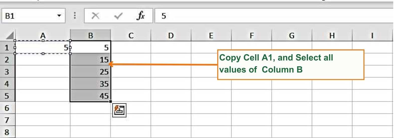
Example 6: In the table image below, we have a value 5 in Cell A1, and subtract it from the range of values given in Column B (B1, B2, B3, B4, and B5)

Here are the simple steps to use ‘Past Special’ features to subtract fixed values from the range of values:

1. Copy the Cell A1 (Press CTRL + C, once to select Cell A1
2. Select all the Cells of column B (B1, B2, B3, B4, and B5)

The Below image shows Copy of A1, and selection of Column B:

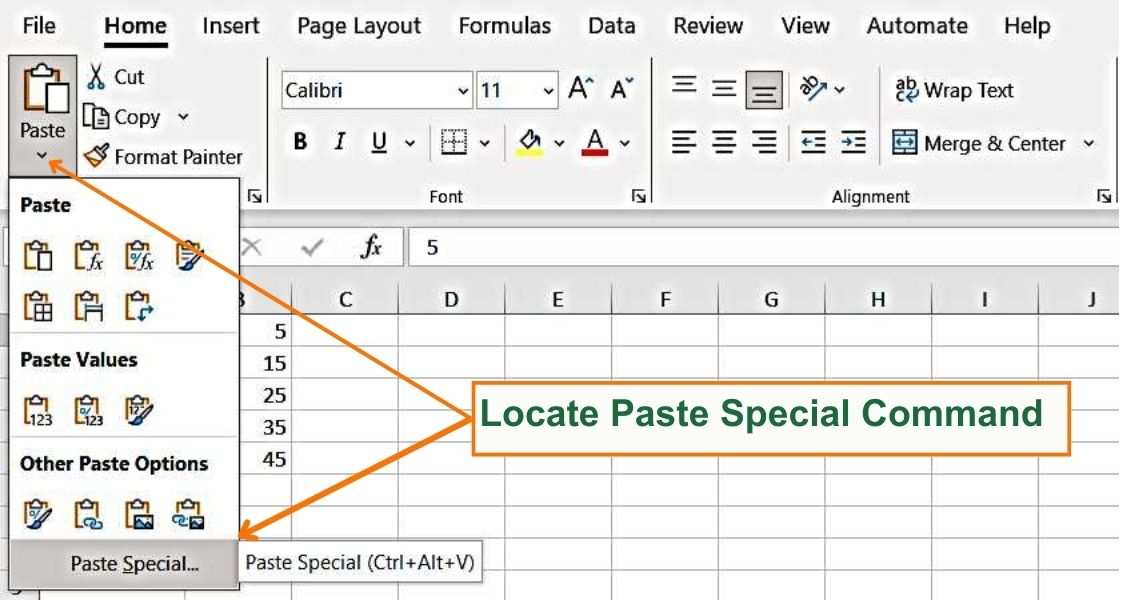
3. Click on the dropdown button of Paste Special and Click on ‘Paste Special’ text. A new window will open.

Paste Special – Step 1: The image below shows how to use Paste Special Command:

3. In the New Window of Paste Special, select the check box against “Subtract.”

Paste Special – Step 2 – Check the box against Subtract: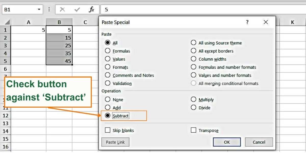

4. Click OK
5. You will notice that all the values in Column B are Subtracted by 5, as we have value 5 in Cell A1.

H. How to subtract Numbers from different Excel spreadsheets within a workbook.

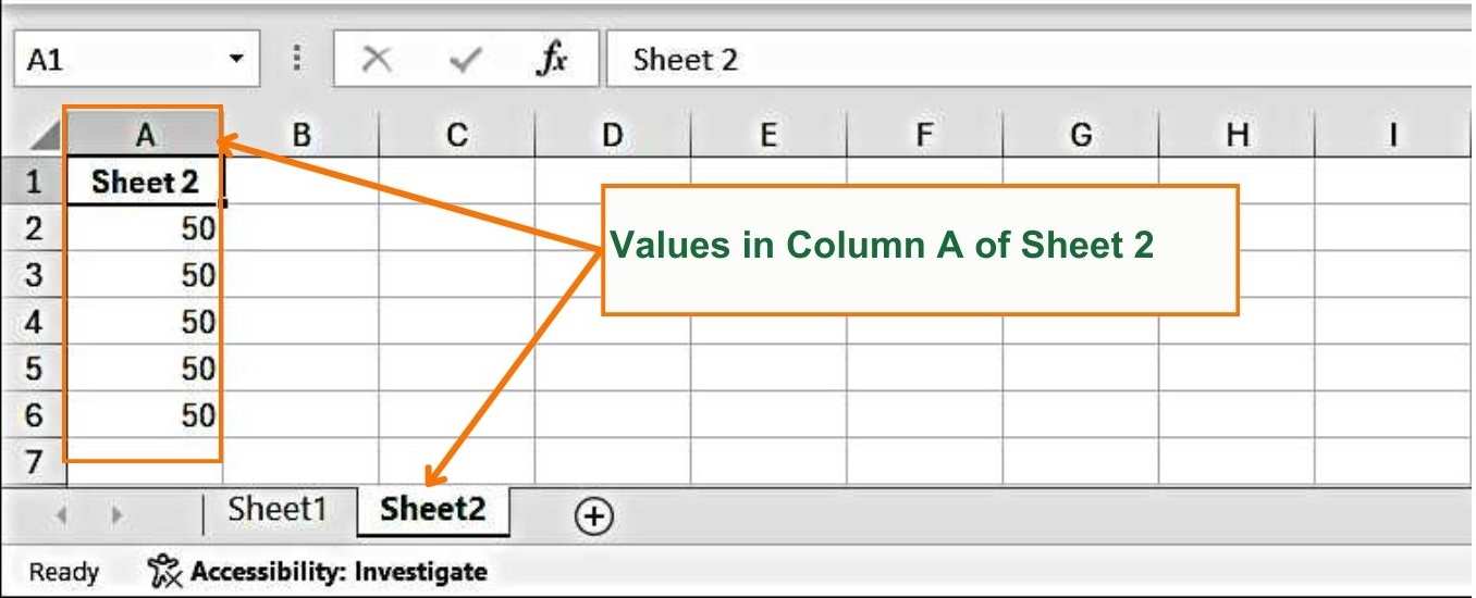
Example 7:  We have Numerical Values in Cells A2 to A6 of Sheet 1, Also we have Numerical Values in Cells A2 to A6 of Sheet 2. Let’s Subtract the values of Sheet B in Column B of Sheet A.

Image H.1 – Values in Sheet 1

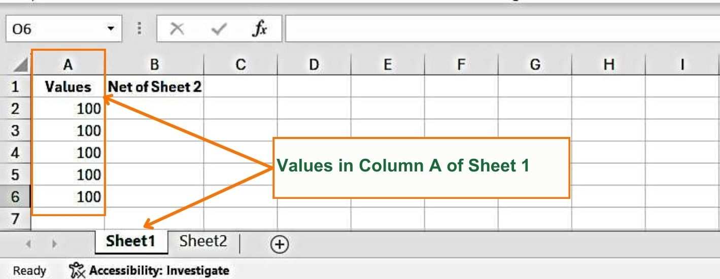
Image H.2.: Numerical Values in Cells A2 to A6 of Sheet 2:

Here are the simple steps to subtract numbers of Sheet 2 from Sheet 1:

1. Go to Cell B2 and Type: =
2. Move the arrow key to Cell A2, and press ‘-‘(Minus). Your formula will look like this: =A1-
3. Go to Sheet 2, select A2, and press ENTER. Now your formula will look like this: =A2-Sheet2!A2

You will get the result in only one cell, that is B2. H.3. See the image below: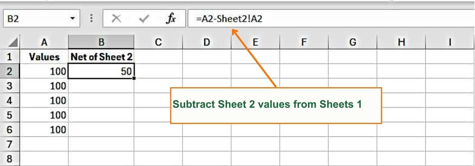

Now you also need results in other cells, B3, B4, B5, and B6. To do this

3. Select cells all the cells, from B2 (That must include the formula calculated in step 2) to B6
4. Press CTRL + D, alternatively you can also copy B2 (CTRL + C) and past (CTRL+V) in cell B3, B4, B5 and B6.

You will get all the values of Sheet 2 subtracted from the values of Column A of Sheet 1.

Image H.4: Shows the subtraction of entire Column A of Sheet 2 from Column A of Sheet 1:

Happy Learning!