How To Multiply in Excel

Introduction:

This Excel Training module educates users on How to Multiply in MS Excel by using various practical examples.

Here are the different approaches to use multiplication in MS Spreadsheet:

A. What is the operator used for Multiplication in Excel?

MS Excel uses Asterisk Sign (*) for multiplying any numbers in the spreadsheet. Whereas in mathematical calculations we normally use the ‘x’ sign for multiplication.

B. What is the function for Multiplication in Excel?

In Excel there is a function available for multiplication called PRODUCT, this is quite often used for the multiplication of a range of numbers.

So, you can use ‘*’ and the PRODUCT function to multiply numbers in Excel.

C. How to multiply in Excel as one would do in calculators.

Example 1: To multiply numbers as one would do in calculators, simply follow the following steps:

1. Go to any cell, Let’s say A1
2. Press ‘=’ sign and press any numbers followed by ‘*’ sign
3. Press another number, if you wish to multiply two numbers. If you want to multiply more than two numbers, then enter ‘*’ and follow it by numbers. Press Enter

See the image below showing the product of 3 Numbers:

D. How to Multiply in Excel using the cell references.

Example 2: To multiply numbers using the cell references we do not have to type the values directly in the formula bar rather we use the cell references.

Here are simple steps to follow:

1. Enter values 2, 3, and 4 in cells A1, B1, and C1 respectively.
2. Go to Cell A3 and Type: =A1*B1*C1, press Enter
3. You will get the answer in Cell A3

The image below shows the multiplication of 3 numbers using the cell references.

E. How to Multiply in Excel using the PRODUCT function.

MS Excel has a function called PRODUCT, to multiply the numbers which means we can also use the function in place of an asterisk sign to multiply the numbers. However, it is used when the multiplication of a range of numbers is done.

Example 3: Let’s have numbers in Cell A1, B1, and C1 and we need to calculate the product of these numbers in Cell C1

Here are the simple steps to follow:

1. Go to Cell A3, and Type – =PRODUCT (A1:C1)
2. Press Enter

Here A1:C1 shows the range of cells, and the PRODUCT function calculates the product (multiplication) of all the values present in the cell ranging from A1 to C1.

The image below shows how to multiply in Excel by using the PRODUCT function:

F. How to Multiply the numbers of one row with another row.

Example 4: We have values in Row 1, in Cells A1, B1, and C1 and there are values in Row 3 in Cells A3, B3, and C3. The product of these cells will be calculated in Row 5

Here are the simple steps to follow:

1. Go to Cell A5, and press ‘=’ followed by A1*A3, (=A1*A3), and press ENTER

2.a. Drag the lower right point of Cell A5 to Cell C5

OR

2. b. Select all the cells from A5 to C5 and Press ‘CRT+R’

The images below Show ‘How to Multiply the numbers of one row with another row’

Image 1

Image 2

G. How to Multiply a single fixed Number with the Column values.

Example 5: Let’s have a sheet where there are values in Cells A1, A3, and A5 (Column A) and We also have a Value in Column B in Cell B1. And we wanted to multiply B1, Fixed Value, with all the values present in Column A (A1, A3, and A5) and calculate the product in Cell C1.

Here are simple steps to multiply fixed values with the Column Values:

1. Go to Cell C1, Type =A1*B1
2. Fix the values of Cell B1 by incorporating dollar sign ($) in the Formula in C1. Change B1 to $B$1.
3. Revise the Formula in C1, new formula is: =A1*$B$1

Keyboard Shortcut to Fix the Cell: In the formula bar click on the Cell that needs to be Fixed (B1 in this example) and Press: the F4 Key

See the image below:

4. Copy the Cell C1 and Paste in the Cell C3
5. Copy Cell C1 and Paste in the Cell C5

Now you have a product of Column A and Fixed Value ($B$1) in Cells of Column C.

See the image below:

H. How to Multiply the Numbers of one column with another column.

Example 6: Let there be numbers in Column A and Column B, and we need to calculate the product in Column C.

Here are the simple steps to do this:

1. Go to Cell C1 and Press ‘=’ sign.
2. Move the arrow key to cell A1, followed by the ‘*’ sign
3. More arrow key to cell B1 and Press Enter
4. Select Cell C1, C2, C3, C4 and C5 and Press, CTRL + D.

This will copy the formula of Cell C1 in the rest of the cells of column C

I. How to Multiply numbers using paste special function.

Paste Special feature in MS Excel is used to multiply the numbers in the spreadsheet without using the Multiply/PRODUCT feature.

Example 7: Let us assume that there are numbers in column A (Cells: A1, A2, A3, A4, and A5) and multiply these numbers with 5 without using the multiplication formula.

Here are the simple steps to follow for using the Paste Special function in Excel for Multiplication:

1. Type Number 5 in any Cell other than which has values, say in Cell E1
2. Copy Cell E1 (CTRL + C)
3. Select all the Cells with Numbers in Column A (A1, A2, A3, A4, and A5). See the image below:
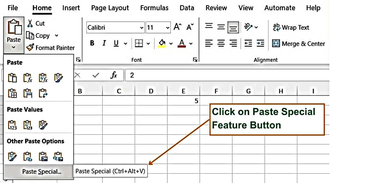
4. Locate Paste Special Feature in the Paste Button dropdown in the Home Ribbon Tab. See the image below:

5. A new ‘Paste Special’ Command will open. Check the Button against the ‘Multiple’ operation and Click OK. The image below shows the ‘Multiply’ Operation in the Paste Special Window.

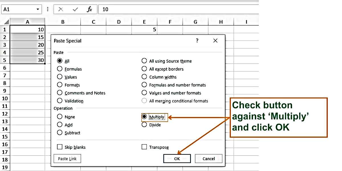
6. You will notice all the cell values (Cells: A1, A2, A3, A4, and A5) get multiplied by 5 automatically.

Keyboard Shortcut to Multiply using paste special: Alt+E+S+M

J. How to Multiply Numbers on one sheet with the numbers on another sheet.

Example 8: Let’s have an Excel Workbook with 2 sheets, Sheet 1 and Sheet 2. In Sheet 1. let us have Numbers in Column A (Cells: A1, A2, A3, A4, and A5), and, we have numbers in Column A (Cells: A1, A2, A3, A4, and A5) of Sheet 2. Calculate the multiplication result in Column C.

Here are the simple steps to perform multiplication across different sheets:

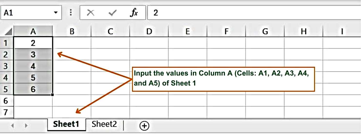
a. Input the values in Column A (Cells: A1, A2, A3, A4, and A5) of Sheet 1. See the image below.

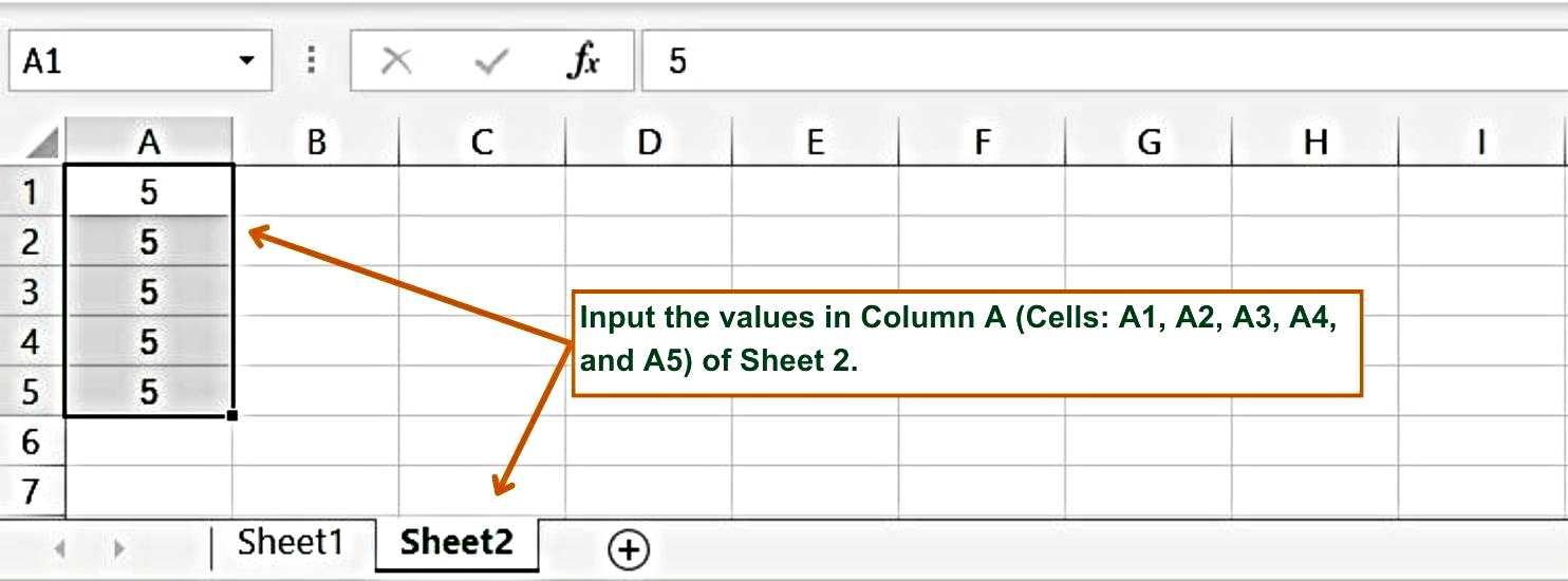
b. Input the values in Column A (Cells: A1, A2, A3, A4, and A5) of Sheet 2. See the image below.

c. Go to Cell C1 of Sheet 1 and press ‘=’ sign.

d. Move the arrow key to Cell A1 of Sheet 1.

e. Press the ‘*’ sign.

f. Go to Sheet 2 and click Cell A1. Press Enter.

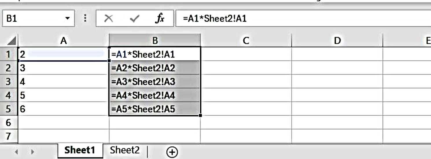
g. Copy Cell B1 to B5, and press CTRL + D

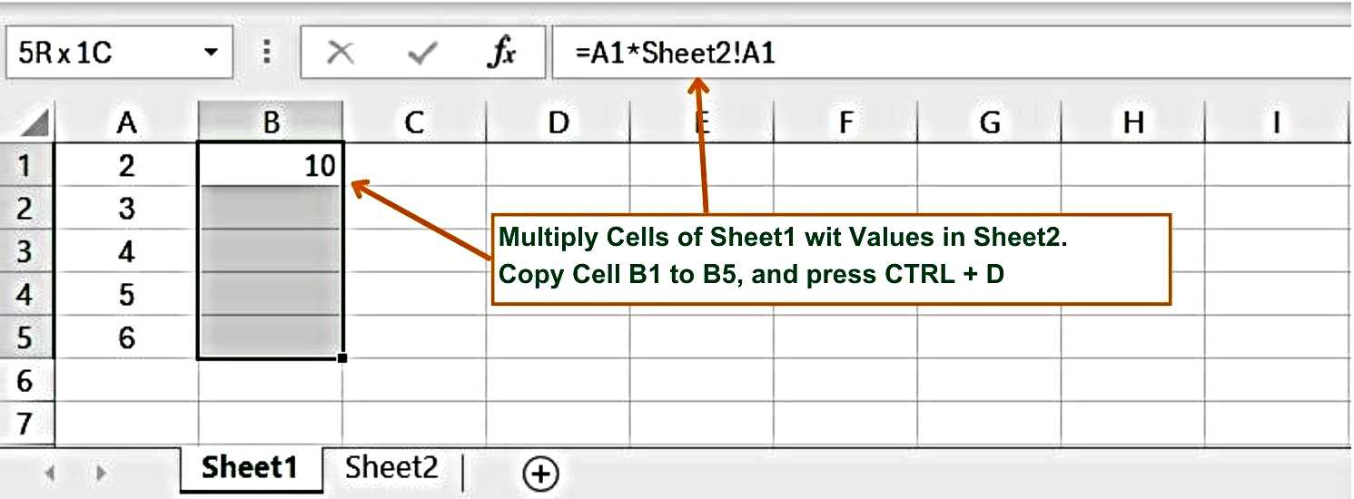
You will notice that the formula in Cell B1 will get copied into all the cells.

K. How to use Multiply and SUM in the same formula.

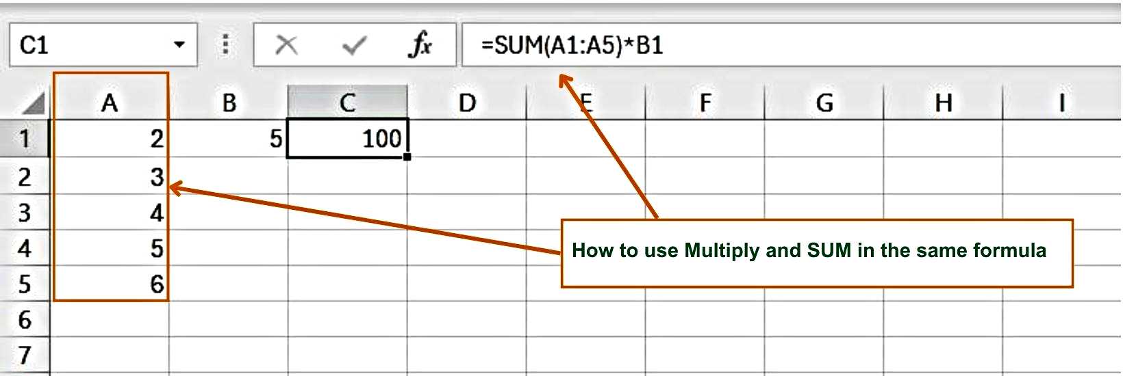
Example 9: Let’s have Numbers in Column A (Cells: A1, A2, A3, A4, and A5) and a number 5 in Cell B1. Calculate the product of SUM of values of column A and Value in B1 in Cell C1.

Here are simple steps to follow:

1. Go to Cell C1 and press ‘=’
2. Type, SUM(A1:A5). This is done to calculate the sum of all the values of column A
3. Press ‘*’ and click on Cell B1. Press Enter

See the image below: