Lookup in Excel (With Examples)

The Lookup in Excel is used in situations where one needs to find specific information from large datasets, which helps in sourcing corresponding values from other columns or rows of the dataset. The Lookup function searches value, called as lookup value, from the reference data set and pulls out the desired value from other Column/Row of that data. It is one of the most widely used lookup and references functions of MS Excel.

Example 1:

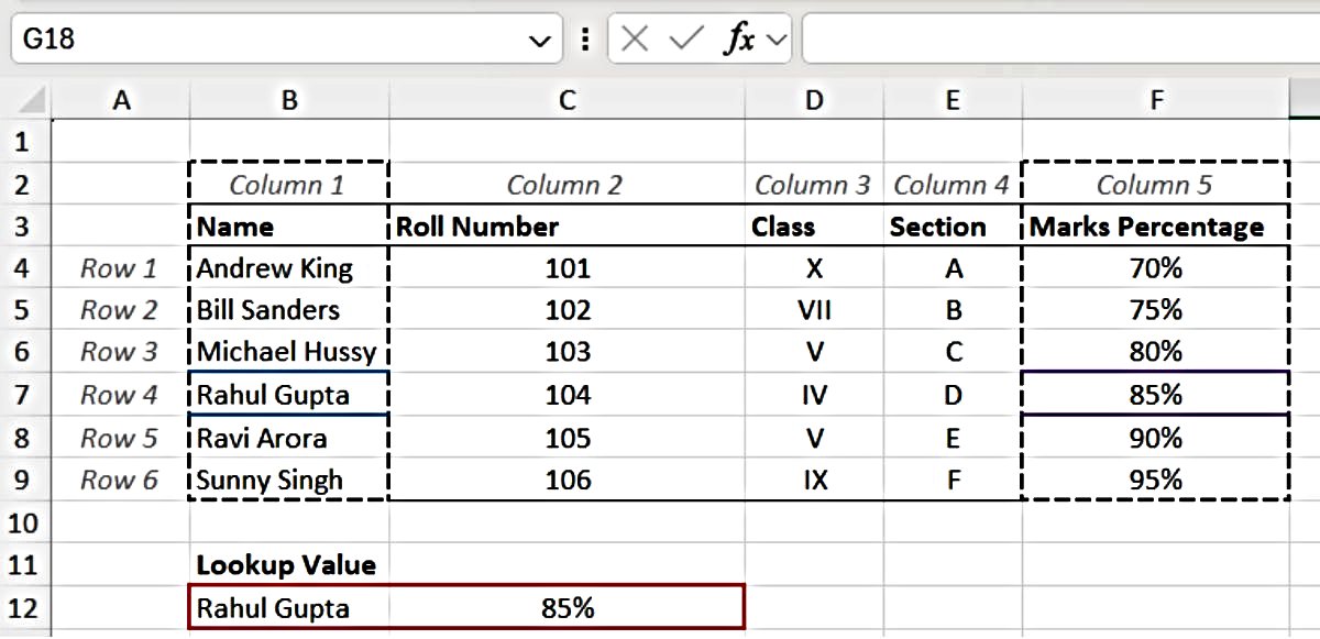
Let us understand Lookup function with the help of an example. For instance, if we have a data set of students of a particular School consisting of Roll Number, Name, Class, Section and Marks percentage. See the data set below:

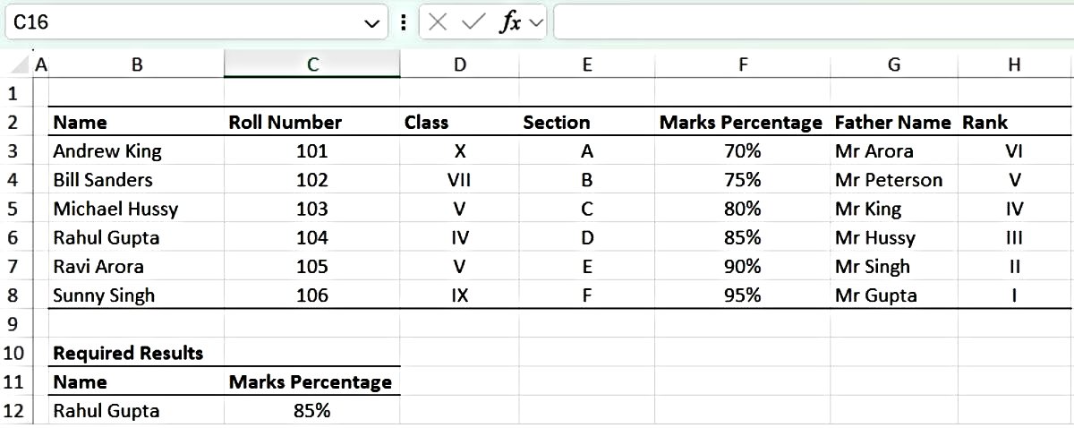
We came across a situation where we need to have mark percentages against each Name. In such cases, we can either manipulate the data and delete all figures except Roll No. and marks percentage OR we can simply do it by using the lookup in Excel and pull up the Students’ name and their marks percentage in another cell.

We will do solve this problem by using the lookup function in this article.

The Lookup function of Excel has two forms, which are used to look up values in the reference data sets. These forms are:

1. Vector form
2. Array form.

Either of these can be used to fetch the percentage marks of students against each name. We will be using each one individually.

*Mandatory Requirements

Please note that it is important, rather mandatory, to sort the reference data in ascending order, that is, from A to Z or from smallest to largest; before using the lookup in Excel otherwise, it will give erroneous results.

The vector form of the Excel lookup function is used to search for specified data either in a one-column range or a one-row range of reference data set and return the value from the corresponding position in another cell.

From the above Example 1, if we need to pull up the Marks percentage of Rahul Gupta, then the vector form would throw the marks percentage from the same row (Row #6) where Rahul Gupta’s name is in the table.

Lookup Vector form for one column range (Vertical Lookup):

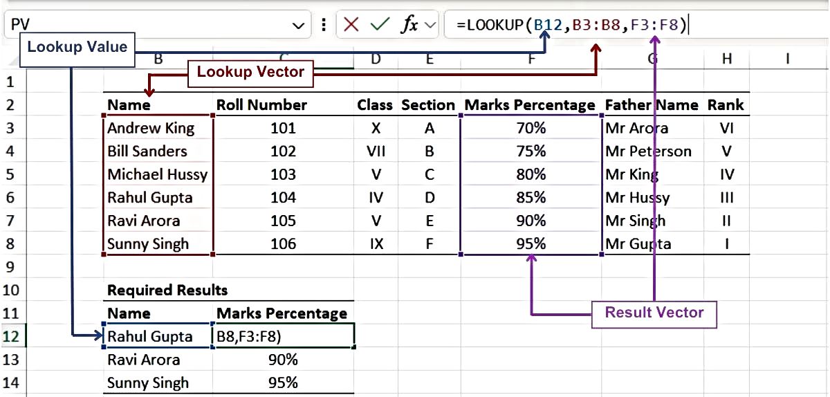
Syntax of Vector Form of Excel Function

In the above example, we could see three things:

1. Lookup Value (Required): Name of student for we need to look data for i.e. Rahul Gupta.
2. Lookup Vector (Required): Column Range from B3 to B8. i.e., a column containing names of students.
3. Result Vector (Optional): Column range where we need to pull results against lookup value. i.e. marks percentage of students.

Here is the Syntax for vector form:

=lookup(lookup_value, lookup_vector, results_vector)

Lookup Vector form for one Row range (Horizontal Lookup):

Example 2:

Let us understand how to use the lookup in Excel with an example. We have the same data set but arranged in a different format; that is, now we have all the column values arranged row-wise.

Let us look for same results, that is Rahul Gupta’s Marks percentage.

Since all the values are arranged row-wise here, we will select the required row range for the lookup vector and range vector.

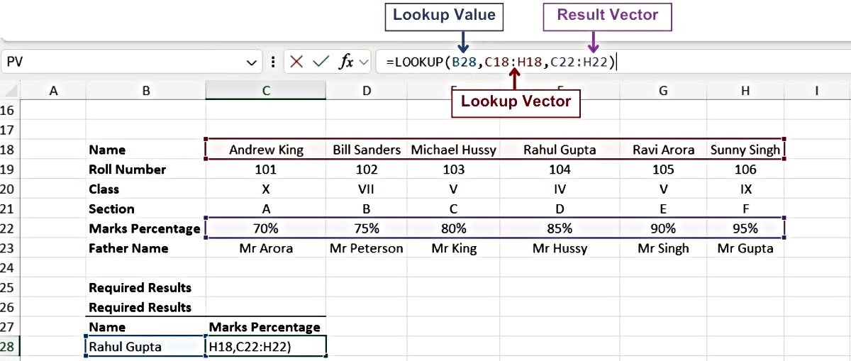
The choice of one-row range or one-column range depends on the arrangement of the data set and our requirements.

Important points to keep in mind while using the Vector Form of the Lookup function in Excel:

1. The range of one-row or one-column of lookup vector and result vector must be of the same size, meaning that if you have selected five rows of column B (lookup vector) then you must select five rows of Column F (result vector). The same applies to a one-row lookup (horizontal lookup).
2. The lookup function works on the principle of approximate results. First, it looks for the exact match, if it does not find the exact result, then it gives the nearest smallest value in its results.
3. The lookup in Excel is NOT case sensitive, which means it doesn’t differentiate textual data, be it in lower case or the upper case; it gives the results based on the value rather than its case.

Error in lookup function:

1. The lookup function in Excel will throw an error in the results, N/A, if the lookup value is smaller than the smallest value in the lookup vector.

Unlike the vector form of Excel lookup, where we use either one-row or one-column to search for the results, in Array form, we use the array range to pull the results.

The Array form of Excel’s lookup function first searches the lookup value in the first column (or Row) of the selected range (An Array) and then throws results from the last column (or Row) of the selected range.

*Important points you need to remember:

1. The data set must be sorted in ascending order otherwise, it may cause errors in the results.
2. If the selected data range (an array) has more Rows than Columns, the Array Form will return results from the last column of the range, corresponding to the same row position as the lookup value in the first column.
3. If the selected data range (an array) has more Columns than Rows, the Array Form will return results from the last row of the range, corresponding to the same column position as the lookup value in the first row.

Let us understand it with the help of an example.

Example 3: Situation 1: Where the array has more Rows (6 rows) than Columns (5 Columns)

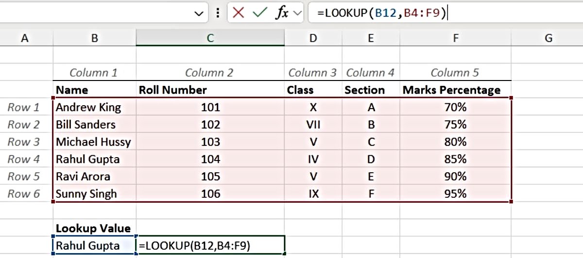
The result below is the array form of the Lookup function, which corresponds to the last Column (column 5) and matches the same row position as “Rahul Gupta” in the first column.

Example 4: Situation 2: Where the array has more Rows (6 rows) than Columns (5 Columns)

We have the same data, except we have inserted an additional row (Row 1) containing data A, B, C, D, E, and F. We have inserted this row to demonstrate that the data in the first row should be sorted in ascending order (A to Z).

In this data table, we have more Columns than Rows, If we apply the Array Form of the lookup function, then it will pull us a result from the last row of the range, corresponding to the same column position as the lookup value in the first row.

In example 4 above, we have used the same array form function as we have used in example 3 (data tables 5 and 6), but here it gives a different result. We have looked up “A” and it gives result as “Rahul Gupta” instead of “F” reason being we have more columns than rows in our Array (data range).

See the results and formula in the image table below.

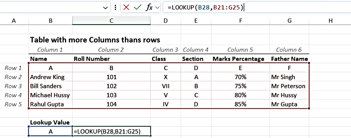
The only difference between Example 3 and Example 4 is the range. In example 3, we have more rows than columns, whereas in example 4, we have more columns than rows.

We have to be careful while using the array form of the lookup function in Excel, as we have to prepare the data before we apply it.

The use of the lookup function is limited in many senses, therefore, it is always recommended to use more advanced lookup and reference functions of Excel in place of the array form of lookup. These functions are:

1. Vlookup: This function looks up a value in the very first column of a selected range of data set and moves on VERTICALLY to return a value in the same row from another column.
2. Hlookup: This function looks up a value in the very first row of a selected range of data set and moves on HORZONTALLY to return a value in the same column from another row.

Microsoft has provided more advanced lookup functions such as Vlookup and Hlookup. However, Microsoft 365 has provided more advanced lookup functions, such as Xlookup, which has overcome the limitations of Vlookup and Hlookup.

Here are some of the advanced types of lookup functions in Excel.

1. Vlookup
2. Hlookup
3. Xlookup
4. Index/Match Functions